Upon arrival in the lab, the sediment cores are sectioned and each section is sampled, thoroughly mixed, and prepared for “grain-size analysis” using the Stoke’s Law equation1 to run the test.

The lab technician pours each sediment sample into a glass column of water (Figure 1), shakes it, and lets the coarse sand and gravel settle out (in about 30 seconds). The tech removes and weighs the coarse fraction and repeats the process with the remaining fine sand fraction (a few minutes wait), the silt fraction (a few hours wait), and the clay fraction. Any idea how long the tech must wait for the clay fraction to settle?

Three days!

It takes clay particles about three days to settle through a perfectly still water column of one ft depth. The deposited clay layer is often very thin – only a fraction of an inch. So, why is this significant in our discussion of “time” as expressed through Earth Science?

Given our example of the engineer’s soil test, how long do you think it took to deposit a 600-4500 feet thickness of clay in the Mancos shale (Figure 2) in an ancient, northwest Colorado shallow sea with currents and water depths of at least 25-100 ft?

Estimates range between 5-20 million years!

These are the types of observations and calculations that led many of the Christian geologists in the early 1800’s to suspect that the earth could be millions of years old.

Example 2: Annual Sediment Deposition Cycles

If you traveled to Alaska, rowed a boat to the center of one of the many lakes, and collected a core of the lake bottom sediment, you might be surprised at what you find. Frequently, you will see many layers of alternating light- and then dark-colored sediment. The dark-colored layers are deposited in the summer months when intense lake vegetation falls to the bottom. The lighter layers are deposited in the winter months with very little organic carbon deposition. Hence, each dark and light couplet reflects one year of sediment deposition within the lake. You simply count each couplet to calculate the age of the lake—similar to counting tree rings. You can occasionally confirm the dates by matching them with thin layers of volcanic ash which fell into the lake during known eruption events (and dates).

Again, the significance?

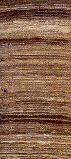
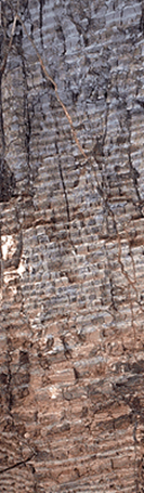
Over 60,000 couplets have been measured in the bottom sediment of Lake Suigetsu, Japan (Figure 3a).

Ancient couplets that are exposed in rock or shale are termed “varves.” Over two million varves are present within the Green River Shale Formation alone (Figure 3b); they reflect two million years of deposition of this one geological unit.

Example 3: Ice Cores

In 1989, an ambitious research project was initiated on the thickest point of ice on the Greenland Ice Cap (termed “GRIP,” aka. Greenland Ice Core Project). The goal of the three-year program was to drill and collect ice cores through the 10,000 ft thick cap. The cores were described, packaged, and shipped for extensive studies of the ice chemistry (Figures 4a and b).²

The center of the cap is an arctic desert with less than five inches of precipitation per year. The scant precipitation produces a thin layer of clear ice in winter; whereas, wind-blown dust creates a dark layer in the summer. This couplet of clear and then dirty ice again represents one annual cycle of deposition (Figure 5). Over 60,000 couplets (years) have been counted, although much older sections (>100,000 years) of disturbed ice are present at the base of the ice sheet.

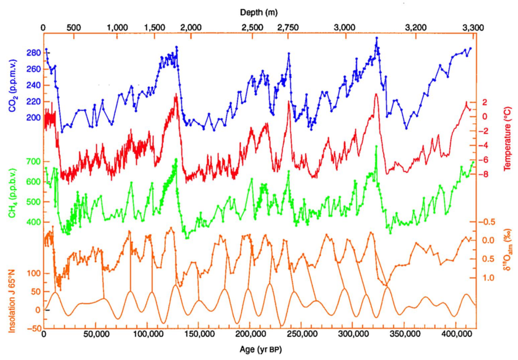
Ice cores were also collected at the Russian Antarctica Base Camp (Vostok) during the 1970s that displayed much older subsurface ice than in Greenland. In 2003, a collaborative effort with French scientists retrieved a core that penetrated 3623 m (10870 ft) of ice with couplets. It included over 420,000 years of preserved record stretching back over the past four glacial periods (Figure 6).³

How do we know that each couplet represents a single year; and, are we sure the cores include no missing or extra couplets?

Great questions.

Again, the most reliable method is to link the numerical sequence of a couplet (its count in years before the present date) against the deposition of a known and dated event that is also recorded in the ice, such as a large, dated volcanic eruption (Figure 7a). Volcanic ash from major eruptions circles the globe in the upper atmosphere and eventually falls to the ground – and on the Greenland and Antarctic ice caps. The largest ash-fall recorded in the Greenland cores occurred 55,000 years ago (see Figure 7b,c). The type and structure of glass shards in the volcanic ash (Figure 8), the shards’ chemical composition, and the ash impacts upon that year’s ice chemistry (for example, the acidity of the ice) are diagnostic indicators of the volcanic source, eruption date, and in some cases, even the specific volcano. Figure 9 shows the excellent correlation between the dates of volcanic acidity peaks in the Greenland ice cores and the known, corresponding eruption dates.4

Finally, other evidence also points to the accuracy of the ice-core couplet dates. Large cycles in CO2 and CH4 concentrations in the Vostok cores occur about every 100,000 years (see Figure 6). These cycles have been linked to the Milankovitch cycles [100,000-year cycles in the slightly elliptical (non-circular) orbit of the earth, at which point the earth is farthest from the sun]5. Hence, the Vostok CO2 and CH4 cyclicity reflect complex climate trends that are also associated with astronomical cycles.

Conclusions

These three examples are a tiny sampling from a myriad of methods that estimate time intervals on earth. Most studies suggest that the earth is millions to billions of years old. [Remember, two of the examples from above (the ice and lake sediment) reflect the ages of surficial material only; the underlying rock strata is much older]. Can you now appreciate the apparent conflict that many Christians associate with scientific methods and their understanding of Scripture? However, “Truth in Scripture” cannot contradict “Truth in Creation.”

Something must be amiss.

Remember, God is the Great Creator! We’ll examine a Creation model in our later lessons that beautifully links the observations of great age in Creation with verses from Genesis 1 that suggest six literal 24-hour creation days. But, just like the engineer’s riverbank example from above, the future model discussions require strong foundational support—we must lay more groundwork.

Next, we’ll turn our attention heavenward to determine the age of the stars and planets as expressed through astronomy in our final discussion in this series on “Time.”

¹Stokes, G. G. (1851). “On the effect of internal friction of fluids on the motion of pendulums”. Transactions of the Cambridge Philosophical Society. 9, part ii: 8- 106. Bibcode:1851TCaPS…9….8S. The formula for terminal velocity (V) appears on p. [52], equation (127)

²Centre for Ice and Climate, Niels Bohr Institute; Stratigraphy and Dating:
https://www.iceandclimate.nbi.ku.dk/research/strat_dating/

³Vostok Station; https://en.wikipedia.org/wiki/Vostok_Station

⁴Centre for Ice and Climate, Niels Bohr Institute; Synchronization of ice cores using volcanic ash layers: https://www.iceandclimate.nbi.ku.dk/research/strat_dating/synch_ice_core_rec/vol_ash_layer/

⁵Milankovitch Cycles; https://en.wikipedia.org/wiki/Milankovitch_cycles

Figure 1. Photo of sediment grain-size analysis in progress. Notice the graduated cylinders in the foreground which contain settling sediments.

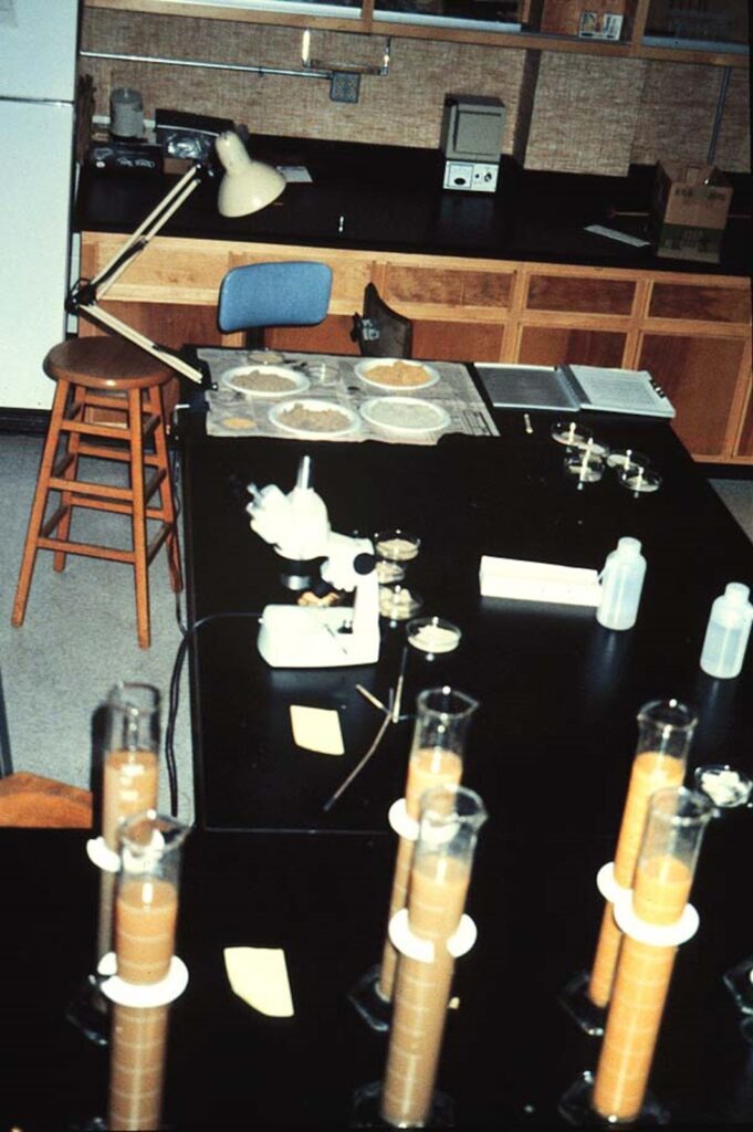
Figure 2. Photo of the Mancos Shale in northwestern Colorado.

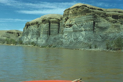
Figure 3a, b.  Example of dark (summer) and white (winter) couplets in lake-bottom sediment, and varved sediment from the Green River Shale.
Fig. 3a – Clay Layers – >60K Couplets Lake Suigetsu, Japan
Fig. 3b – Varved Shale

Figures 4a and b. Location of GRIP research study in Greenland. Also shown is an ice core segment being inspected and prepared for sampling and/or transport.

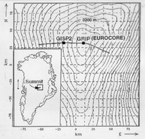
Figure 5. Close-up view of summer (dark) and winter (light) ice from the GRIPd cores. Each couplet reflects one-year of ice deposition.

Figure 6.
420,000 years of ice core data from Vostok, Antarctica, research stations. Current period is at left. From bottom to top: insolation at 65 Degrees North due to Milankovitch cycles (connected to ¹⁸O).¹⁸O isotope of oxygen; levels of methane (CH₄); relative temperature; levels of carbon dioxide (CO₂).

Figures 7a, b, c.  Volcanic eruption, and example of significant ash layer in GRIP ice core.

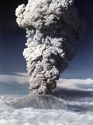
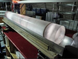
Figure 8.  Volcanic ash shards collected from ash layer in GRIP core.